
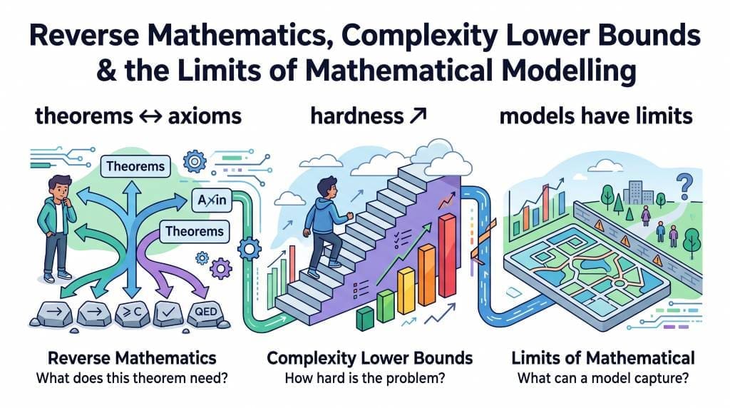
A weather app processes millions of data points before breakfast, while logistics companies reroute trucks overnight and hospitals use models to spot potential outbreaks early. Yet, all these tools rely on one big assumption: that their calculations will finish on time. But what happens when they don’t? A model might run all night without finding an answer, a solver might return no result, or a proof might remain unfinished. We often blame the code, but sometimes the real problem lies in the task itself. Researchers have shown that some problems are inherently difficult to solve efficiently. This is where computational hardness in models comes in, helping us understand why some calculations take so long and where mathematical models reach their limits.

Complexity lower bounds then pose a second question: What is it that no fast algorithm could possibly achieve? Because of this, these two areas establish the true boundary of mathematical modelling. This guide shows that boundary by means of open-access research and simple examples.
Bridging: Why Modelling Has Limits and Why That Matters
Every mathematical model starts with assumptions. For example, climate models assume that physical laws stay consistent, epidemic models estimate how people come into contact, and pricing models often assume that markets have enough buyers and sellers to support trading. We can adjust some assumptions without ruining a model, but others place much stricter limits on what it can do. In fact, some problems may be too difficult for any fast algorithm to solve, no matter how clever the approach. Reverse mathematics complexity lower bounds help researchers explore these limits by examining which mathematical axioms a theorem needs and how difficult it may be to prove.
Complexity Lower Bounds and Computational Limits
Complexity lower bounds show how much extra effort a problem requires and, more importantly, which tasks may resist fast solutions. A modeler who fails to take these limitations into account is chasing answers that are impossible to achieve; on the other hand, one who does take them into account designs wiser tools. The ideas in this article also connect to real-world applications, with further insights available in our advanced research hub and our explainer on the theoretical foundations of computation.
How Reverse Mathematics Explains Proof Complexity
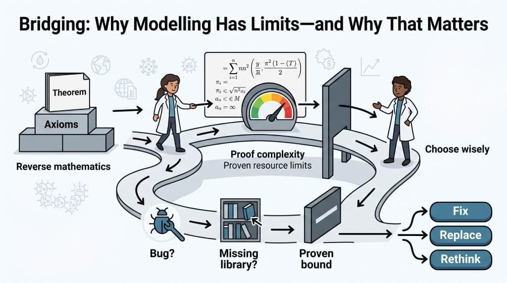
Different problems need different solutions. You can fix a software bug or install a missing library, but a proven lower bound points to a deeper limit that you cannot easily overcome. So, how do we tell the difference? The reverse mathematics of complexity lower bounds helps answer this question by showing which mathematical assumptions a proof depends on. Proof complexity takes this further by examining how difficult a proof is to build. In practice, that difficulty can affect the time and memory a computer needs to solve a problem. In this guide, we’ll explore the process step by step. First, we’ll look at the main subsystems of reverse mathematics. Next, we’ll examine the barriers that limit proofs, see why real-world solvers sometimes struggle to make progress, and finally, turn these ideas into practical methods you can use.
The explanation of software limitations deals with the engineering aspect, while the section on machine-learning alternatives covers the data-driven aspect. Read those two articles next since they finish off the map that this guide initiates.
What Is Reverse Mathematics? A Modeler’s Introduction
Reverse mathematics started with a reversed kind of question. Instead of beginning with axioms as most mathematicians do, Harvey Friedman reversed the direction of the approach in the 1970s and asked which axioms a theorem actually requires. The procedure involves a straightforward reversal: you first take the theorem as a given and then prove the axiom from the theorem. If the axiom matches, it means that the theorem really needs that particular axiom.
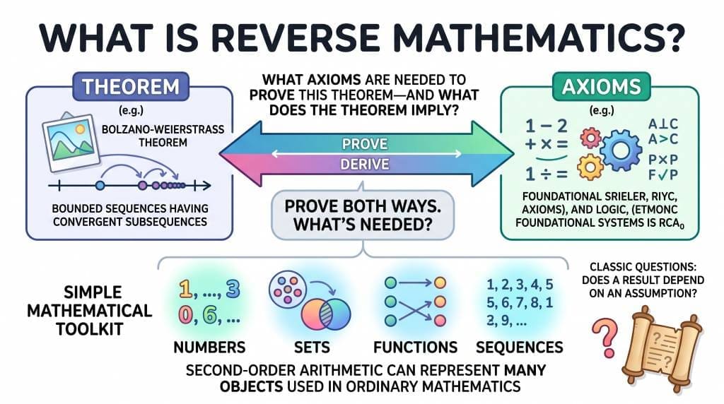
The Stanford Encyclopedia of Philosophy gives an account of this history and links the method to the parallel postulate as well as to the axiom of choice. In those classic instances a direct question was posed: does this statement need that assumption? Nowadays, reverse mathematics is carried out within second-order arithmetic, in which the reals, functions, and sequences are represented as sets. This one step encompasses most of ordinary mathematics.
Reverse Mathematics as an Axiom Audit for Models
During a graduate modelling seminar, I once showed a graph with a sharp bend. The students expected a smooth curve, so I placed a step function beside it. One student then asked, “Which assumption did we break?” The room fell silent for a moment. I explained that this question has a formal mathematical basis. We can treat it as an axiom audit: first, identify the set-existence axioms a model relies on, then determine which of those axioms the result actually needs. This approach connects to the reverse mathematics of complexity lower bounds, which helps us examine the mathematical foundations behind the limits of proofs and models. The answers often fall into a few well-known categories, each linked to a different level of mathematical strength.
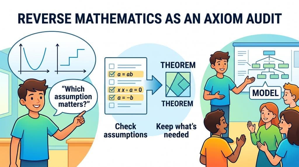
Those students who become familiar with the categories alter the way they construct their models. They cease to add assumptions out of habit and only include what the result actually demands. This kind of discipline applies directly to programming and also to peer review. A modeller who names her axioms can therefore defend her results with confidence.
RCA0, WKL0, and ACA0: Reverse Mathematics in Plain Terms
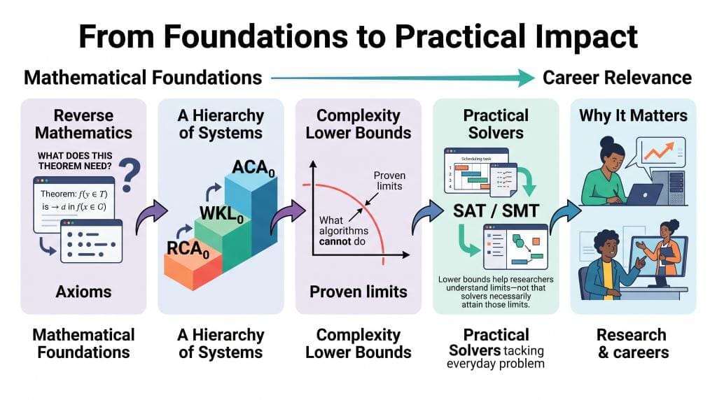
Three main systems do much of the work in reverse mathematics. First, RCA₀ provides a basic foundation for computable mathematics and supports reasoning about objects that can be constructed using limited computational methods. Next, WKL₀ adds a principle called Weak König’s Lemma, which states that every infinite, finitely branching binary tree has an infinite path. This one addition is enough to prove many important results, including the Heine–Borel theorem and the completeness theorem for first-order logic. Finally, ACA₀ allows the construction of sets defined by arithmetic formulas, making it possible to prove stronger results in areas such as real analysis.

Together, these systems help researchers explore the reverse mathematics of complexity lower bounds by identifying the mathematical principles needed to establish particular results.
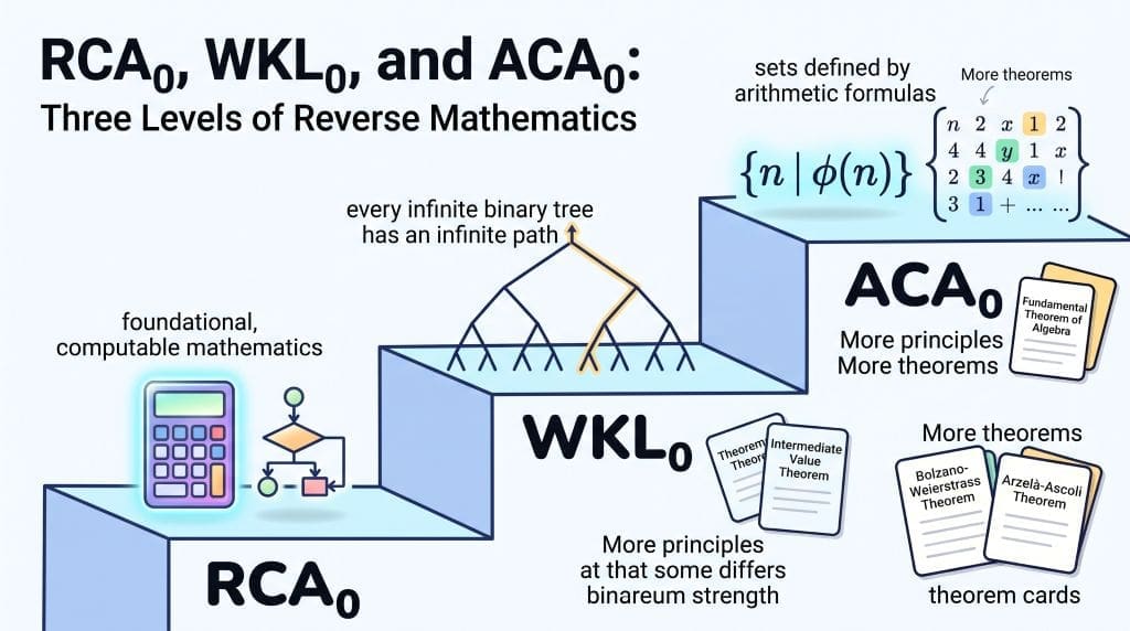
Simpson’s standard work, Subsystems of Second Order Arithmetic, provides a complete account of the entire hierarchy. Normann and Sanders have shown that the Big Five continue to organize the field, and their more recent work extends into second-order and higher-order settings. However, applied modellers seldom need anything beyond the first three levels.
Proof Complexity, Bounded Arithmetic, and Complexity Lower Bounds
Proof complexity studies how large or difficult a mathematical proof must be. Checking a short proof usually takes little effort, while finding a long one can require much more time and computing power. One of the best-known systems in this field is resolution, which plays an important role in SAT solvers. However, resolution struggles with certain problems, including the pigeonhole principle. In particular, proving that more pigeons than holes cannot fit into the available holes requires exponentially many steps in standard resolution proofs. This is not a software bug or a flaw in the solver. Instead, it is a proven lower bound that reveals a limit of the proof system.
Such results are important to the reverse mathematics of complexity lower bounds, which explores the mathematical foundations behind the limits of efficient proofs and computation.
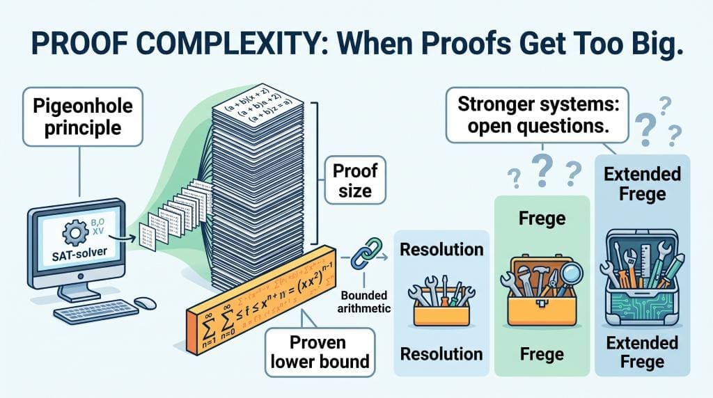
Frege systems are more powerful tools, and extended Frege systems are even more powerful than that. We still do not have sharp lower bounds for these systems. This open problem stands alongside the question of whether P equals NP. Bounded arithmetic provides the logical connection between proof length and computational difficulty. In his 2019 book, Proof Complexity, Krajíček fully develops this framework. These results make proof size a first-class modelling constraint.
Resolution, Frege, and the P versus NP Connection
Resolution is easy to picture: a solver combines logical clauses until it finds a contradiction. However, some formulas make this process much harder than others. The pigeonhole principle is a classic example because it requires exponentially large proofs in resolution. Mathematicians have proven this lower bound, so it reflects a fundamental limit of the proof system rather than a problem with its implementation. As a result, SAT solvers can struggle with certain inputs even when they work correctly. Frege proof systems, on the other hand, can use any well-formed formula as a step in a proof, which helps them overcome some limitations of resolution.
These differences matter when studying the reverse mathematics of complexity lower bounds, because they help researchers understand why some proofs demand far more computational effort than others.
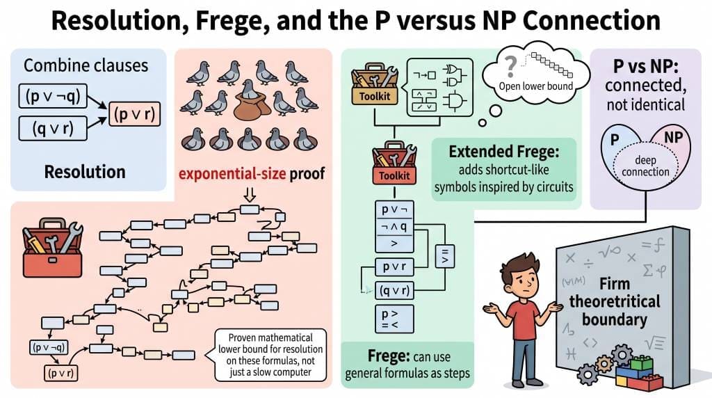
In some instances, a stronger logic leads to shorter proofs. Extended Frege includes a kind of shortcut similar to that used in circuits. However, no superpolynomial lower bound is currently known for it. The absence of this proof stands alongside the problem of P versus NP. Progress on one of these problems would have a significant impact on the other. To sum up, the lower bounds in this area can be seen as negative modelling results.
The Reverse Mathematics of Complexity Lower Bounds
New results have succeeded in bridging the gap between logic and complexity. Chen, Li, and Oliveira investigate which weak axioms are capable of proving various lower bounds, and their ECCC report provides the answer within the framework of bounded arithmetic. Taking Cook’s theory PV1 as a starting point, lower-bound statements are transformed into combinatorial principles. The weak pigeonhole principle keeps reappearing.
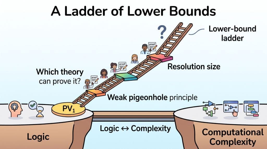
A lower bound thus acquires the status of an axiom by itself, its strength corresponding to that of a known counting principle. Li and Oliveira continue along this line of inquiry by proving that APC1 cannot establish strong separations. Pich and Santhanam then provide a corresponding feasible-provability result. Li, Li, and Ren go on to identify the exact theory concerned with resolution size bounds. Consequently, lower bounds can now be viewed as forming a ladder of axioms.
What Complexity Lower Bounds Mean for Real-World Models
The implications of complexity lower bounds go well beyond the seminar room. When a modeller uses a SAT solver on a difficult formula, the solver responds with a long period of silence. This delay can be linked to a proven resolution bound. The model is not faulty; the problem itself is fundamentally difficult.
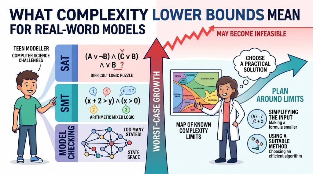
SMT solvers combine arithmetic with propositional logic and extend SAT by incorporating richer theories. With this increased power comes a cost. Many fragments of SMT lie within NP or PSPACE. Model checking encounters the same limitation and, in the worst case, has to search through exponential spaces. The Simons Institute gives a clear explanation of this limitation. Lower bounds show the boundary of what is feasible. Those who study this map are therefore able to plan much more effectively.
SAT, SMT, and Complexity Lower Bounds in Practice
Modern SAT solvers work behind the scenes to solve complex problems. They can process millions of clauses and help engineers verify circuits or plan schedules. However, these solvers can slow down dramatically when they encounter difficult formulas, such as those based on the pigeonhole principle. One reason is that resolution size lower bounds show how large a proof must be. A solver cannot simply skip the steps needed to produce a valid proof. Similarly, SMT solvers handle a wider range of problems by including theories such as linear arithmetic.
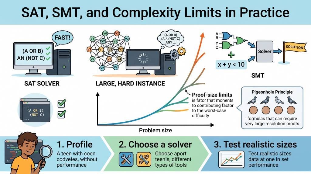
This added flexibility helps them solve more types of problems, but it can also increase computational costs. As a result, even a simple-looking model may time out as the problem grows. So, start by profiling your problem, choose a suitable solver, and then consider the limits of the problem size. A model with a hundred variables might finish in seconds, while one with a thousand could take far longer—or fail to finish within a practical time limit. Understanding these limits is central to the reverse mathematics of complexity lower bounds, which helps explain why some computational problems resist efficient solutions.
Differential Equations and Intrinsic Hardness
Ordinary differential equations are used to model the world around us; they can be employed to study epidemics, electric circuits, and orbits. A symbolic solver might fail when faced with a difficult ODE. In that case, is the problem due to a weak tool or is the equation itself hard? Bournez and Núñez provide an answer using reverse mathematics. They place initial value problems into the Big Five levels.
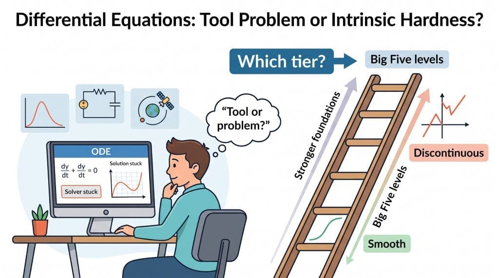
The tier to which the problem belongs is determined by the regularity of the right-hand side. Polynomial maps that are smooth occupy the lower rungs of the scale, while discontinuous maps end up much higher up and some even reach transfinite computation. As a result, one obtains a diagnostic that does not rely on a specific representation. A solver can fail for a logical reason, and that reason is frequently not a technical deficiency. Engineers thus being able to look at the tier before attributing the failure to the code.
Trust, Uncertainty, and the Human in the Loop
There are also established models concerning human trust in automation. Rodriguez and his colleagues have looked at this area. In their paper in Frontiers in Neuroergonomics they outline the limitations. Although conceptual models are comprehensive they are difficult to measure. Mathematical models do provide dynamic elements but require validation. The authors advocate the use of mixed timescales and physiological data. The same level of openness should apply to policy models.
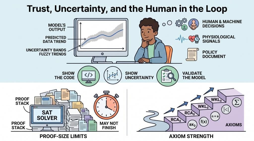
Lo and his colleagues have examined the WHO guidelines. They looked at the way modelling evidence was incorporated into these guidelines. The quality of the studies varied greatly. Very few of them made their code available or provided complete uncertainty ranges. NIST also promotes this standard when it comes to simulation. Good models should include their own error bars.
Two walls matter most in practice:
- Walls of proof size; lower bounds on resolution account for the fact that some SAT runs never come to an end.
- Walls at the axiom level; in order for a solver to have any chance of completing a proof, it may be necessary to use WKL0 rather than just RCA0.
Bridging Pure Logic to Applied Practice
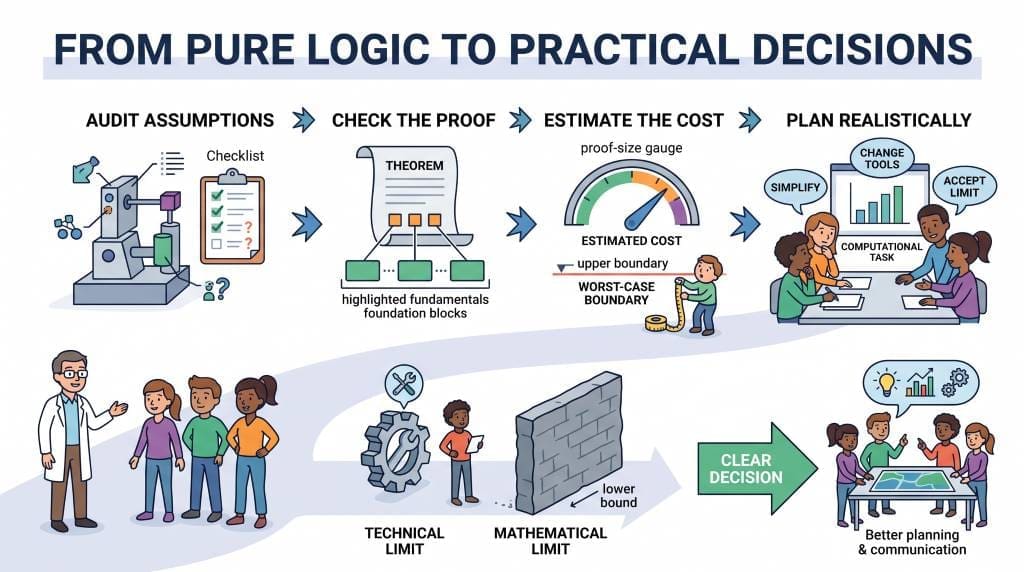
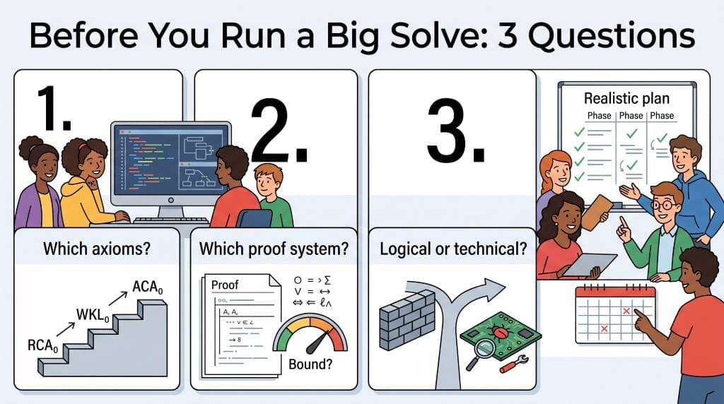
The way you design changes when you know a lower bound. Begin with an axiom audit by writing down all the assumptions your model makes. Then consider which assumption leads to a particular result. Reverse mathematics provides you with that practice whenever you need it. After that, assess the proof by assigning it a price. The lower bound shows you the worst-case scenario and enables you to size the instance appropriately. Simplify only in cases where the logic permits you to. You cannot move a fundamental boundary, but you often can move a technical one. Software limits are different from mathematical limits. Our article on software limitations deals with the first type, while our note on machine-learning alternatives covers the second. Before you refactor, read the proof tier because that habit prevents weeks of wasted computing power.
How Lower Bounds Improve Leadership and Planning
The skills gained accumulate over the course of a career. Organizations employ individuals who are able to say no supported by evidence, with the strongest kind of evidence serving as a lower bound and turning what could be a lengthy discussion into a matter of arithmetic. Data scientists who understand proof complexity are better able to set realistic deadlines. Research leaders who check axioms end up deploying safer models. Funders tend to reward honest scope and clear boundaries. Although the advantage is real it remains unobtrusive. One must become thoroughly familiar with the different levels before explaining them in simple terms. When a group of engineers hears someone refer to the wall by name, they will remember that person. In short, having a solid foundation of knowledge is equivalent to showing leadership, and that individual is the one who is given the next difficult problem.
Verified Resources: Key Papers and Further Reading
- Stanford Encyclopedia of Philosophy — Reverse Mathematics (Eastaugh, 2024), Stanford University.
- Simons Institute — Research Vignette: Lower Bounds in Computational Complexity (Santhanam), UC Berkeley.
- NIST — On Methods of Uncertainty Quantification in Computational Modeling and Simulation (Srinivasan, 2026).
- Epidemics — Contribution and quality of mathematical modeling evidence in WHO guidelines (Lo et al., 2022), peer-reviewed, open access.
- Frontiers in Neuroergonomics — A review of mathematical models of human trust in automation (Rodriguez Rodriguez et al., 2023), peer-reviewed, open access.
- Springer Handbook — Reverse Mathematics (Stillwell, 2024), peer-reviewed chapter.
How This Guide Was Compiled
I put this guide together from the perspective of a physicist who develops and checks mathematical models. First, I reviewed each linked source and checked its DOI metadata through Crossref. I also consulted publisher pages whenever they were available. To keep the information reliable, I based factual claims on peer-reviewed research and government sources, while using newer arXiv and ECCC preprints to explore emerging ideas. I clearly labelled these preprints in the references. In addition, I used older sources only for established background knowledge. Every specific result links to a listed source, rather than relying on unsupported claims. Finally, I used clear language, active voice, and a natural placement of the focus key phrase throughout the headings and text to help readers understand the topic without keyword stuffing.
Frequently Asked Questions
It audits which axioms a theorem truly needs. You prove the theorem first, then prove the axiom back from it.
They are proofs that no fast algorithm can solve a task. In short, they define the boundary of what is feasible.
They tell you when a stall is fundamental. As a result of this, you stop chasing impossible answers.
RCA0, WKL0, ACA0, ATR0, and Π¹₁-CA0; the first three include most of the work that is applied.
Yes. The peer-reviewed DOIs listed here are open access, and the preprints are free to read.
References
- Bournez, O., & Núñez, A. (2026). Relating the computational and logical difficulty of solving ODEs: From polynomial to discontinuous right-hand sides. arXiv. https://arxiv.org/abs/2605.07128
- Chen, L., Li, J., & Oliveira, I. C. (2024). Reverse mathematics of complexity lower bounds (Technical Report TR24-060). Electronic Colloquium on Computational Complexity. https://eccc.weizmann.ac.il/report/2024/060/
- Eastaugh, B. (2024). Reverse mathematics. In E. N. Zalta & U. Nodelman (Eds.), The Stanford Encyclopedia of Philosophy (Summer 2024 ed.). Stanford University. https://plato.stanford.edu/entries/reverse-mathematics/
- Li, J., & Oliveira, I. C. (2023). Unprovability of strong complexity lower bounds in bounded arithmetic. arXiv. https://arxiv.org/abs/2305.15235
- Li, J., Li, Y., & Ren, H. (2024). Finding bugs in short proofs: The metamathematics of resolution lower bounds. arXiv. https://arxiv.org/abs/2411.15515
- Lo, N. C., Andrejko, K., Shukla, P., Baker, T., Sawin, V. I., Norris, S. L., & Lewnard, J. A. (2022). Contribution and quality of mathematical modeling evidence in World Health Organization guidelines: A systematic review. Epidemics, 39, 100570. https://doi.org/10.1016/j.epidem.2022.100570
- Normann, D., & Sanders, S. (2022). The biggest five of reverse mathematics. arXiv. https://arxiv.org/abs/2212.00489
- Pich, J., & Santhanam, R. (2021). Strong co-nondeterministic lower bounds for NP cannot be proved feasibly. In Proceedings of the 53rd Annual ACM Symposium on Theory of Computing (pp. 223–233). ACM. https://doi.org/10.1145/3406325.3451117
- Rodriguez Rodriguez, L., Bustamante Orellana, C. E., Chiou, E. K., Huang, L., Cooke, N., & Kang, Y. (2023). A review of mathematical models of human trust in automation. Frontiers in Neuroergonomics, 4, 1171403. https://doi.org/10.3389/fnrgo.2023.1171403
- Sanders, S. (2013). Reverse-engineering Reverse Mathematics. Annals of Pure and Applied Logic, 164(5), 528–541. https://doi.org/10.1016/j.apal.2012.11.006
- Santhanam, R. (2019). Research vignette: Lower bounds in computational complexity. Simons Institute for the Theory of Computing, UC Berkeley. https://simons.berkeley.edu/news/research-vignette-lower-bounds-computational-complexity
- Srinivasan, V. (2026). On methods of uncertainty quantification in computational modeling and simulation: Harmonizing modeling and metrology practices (NIST AMS 100-85). National Institute of Standards and Technology. https://doi.org/10.6028/NIST.AMS.100-85
- Stillwell, J. (2024). Reverse mathematics. In Handbook of the history and philosophy of mathematical practice (pp. 1963–1988). Springer. https://doi.org/10.1007/978-3-031-40846-5_43