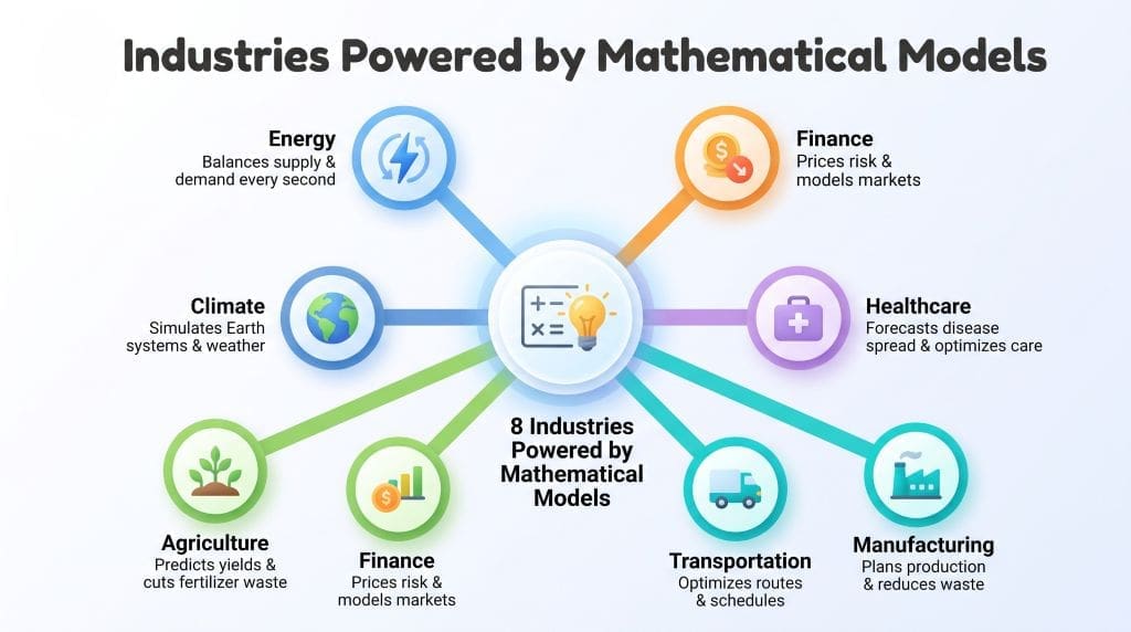

You check the weather app before you head out. Then you glance at a traffic map to dodge the slow route. Later you look at vaccine trial numbers before you decide on a shot. Each of these tools runs on equations. Yet each one uses a different kind of mathematical model. Choose the wrong type and the answer goes wrong. No amount of careful math fixes a mismatched model. So it helps to know the main types. Some deal with certainty. Others include chance. Some track change over time. Others give you a fixed snapshot. Each one answers one specific question. This guide walks through the different type of mathematical models. You will see what each assumes and what it costs. By the end you can match a real problem to the right tool. Start with the correct category and you save both time and money.

Why Choosing the Right Model Class Shapes Real Decisions
The idea of sorting may sound academic, but it has a real impact on the decisions made. A hospital planner requires a different kind of math from a designer. While the planner is concerned with risk and capacity, the designer is more interested in smooth motion and speed. At bottom, it’s the same tools being used, but with different assumptions. Choosing a class is in effect choosing your assumptions. In fact, the choices you make determine what you trust. For this reason, I ask my students early on what your model must get right.
For example, the kind of answer they give will show you the appropriate family. If timing is important, then they will need a dynamic form; when people are involved, they are likely to need agents. By contrast, a simple average is seldom enough. As a result, this habit avoids weeks of rework and also makes the results easier to justify. Begin every project by asking that question. At the same time, having a clear goal helps to keep you focused. Vague answers indicate that the goal is not clear. To sum up, clarity should come before software.
Empirical vs. Theoretical Types of Mathematical Model
Theoretical Type of Mathematical Model
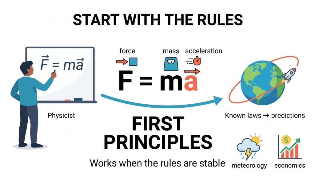
Theoretical models begin with physical laws rather than with data; the physicist then formulates a rule and solves it. A good example is Newton’s second law. The equation F = m a connects force and acceleration. Obviously, none of this is based on a spreadsheet. In fact, each term has a physical significance. This approach is applicable whenever the rule is known. Researchers call this method first-principles modelling. Generally speaking, such models go beyond the data available. In effect, they can also reveal underlying assumptions. As a result, studies on teaching have found that students’ thinking is improved. It is true that constructing such a model requires knowledge of the subject area. A good example is the orbit model, which tracks the planets without referring to any measured table.
This ability is the reason why physicists place trust in theory before data. Both meteorology and economics make use of the same principle. This approach is beneficial in general whenever the rules remain stable.
Empirical Models Built From Data
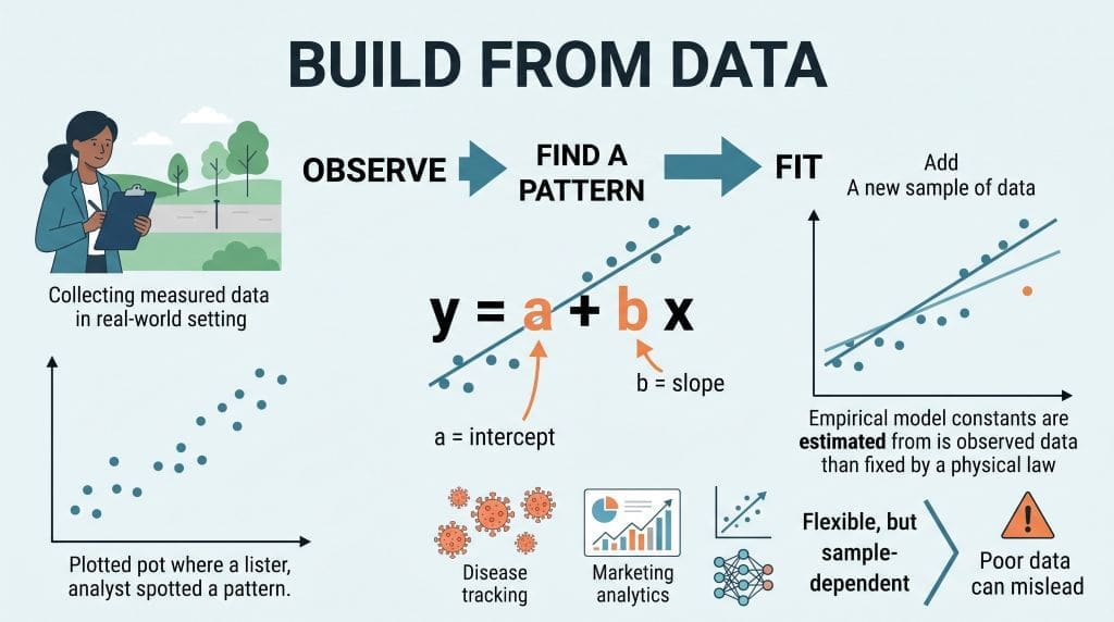
Empirical models start by using readings. To do this, an analyst gathers some numbers and looks for a pattern.
For example, a straight line follows the equation (y = a + bx). In this equation, a stands for the intercept and b for the slope. In reality, scientists adjust the constants to match the data that they have observed. Nature does not determine the values of these constants. As a result, the model fits very closely to one particular data set. A new sample could cause all the values to change. Indeed, disease teams make use of this approach.
A general examination of pandemic models shows that this trend exists. Ultimately, both regressions and neural networks follow the same route. Overall, the advantage of this method is its flexibility. On the other hand, its disadvantage is that it depends on the sample. For instance, marketing analytics make use of such fits. Of course, how researchers collect the data affects the quality of the results. Poor samples lead to confident nonsense.
Choosing Between Theory and Data
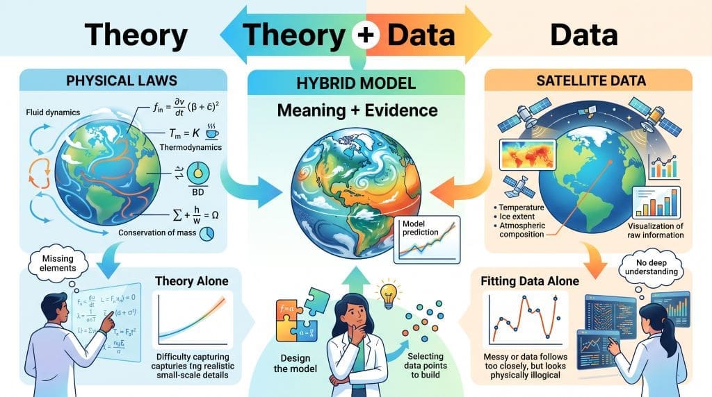
In reality, the majority of projects combine both methods. For example, theory provides the basic framework; climate science is a good illustration of this. Generally speaking, the physical laws control the way fluids flow. The satellite data is then used to determine the uncertain parameters. Consequently, the model remains clear and well-founded. Relying solely on theory may fail to take account of the complexities found in the real world.
A pure fitting approach might overlook obvious physical principles. In fact, good modelers begin by examining both possibilities. To that end, they first consider which equations need to be explained and then see what numbers the data gives. Briefly put, the decision involved is a matter of design. This practice avoids wasting weeks later on later work. Overall, a hybrid model is better than either of the two extremes because it retains meaning while taking in new evidence. Students acquire this balance through hands-on experience. In fact, textbooks omit the complicated middle section. Of course, that is where actual work takes place. Making clear choices has benefits in the long run.
Stochastic vs. Deterministic Types of Mathematical Models
Deterministic Type of Mathematical Model
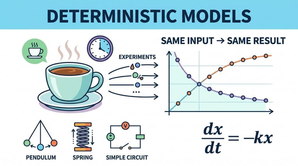
Deterministic models produce the same result for a given input since nothing within them depends on chance. For instance, a differential equation expresses the dynamics involved; one typical form is d x / d t = -k x, an equation which can be used to describe cooling and decay. Moreover, if the experiment is repeated, the same curves are obtained. Engineers appreciate this kind of predictability when carrying out design work. I once saw a class in which they were modelling the cooling of coffee and each group obtained the same curve. Furthermore, the fact that the results were identical made it easy to talk about physics. Initially, the equation revealed nothing to the students. On the other hand, a major drawback is that it lacks surprise.
Real systems almost never behave in such a simple and neat manner. In fact, both traffic flow and pendulums belong to this category. Of course, simple circuits and springs do too. Deterministic mathematical models form the basis of classical mechanics and are in general the natural starting point.
Stochastic Model Driven by Random Variables
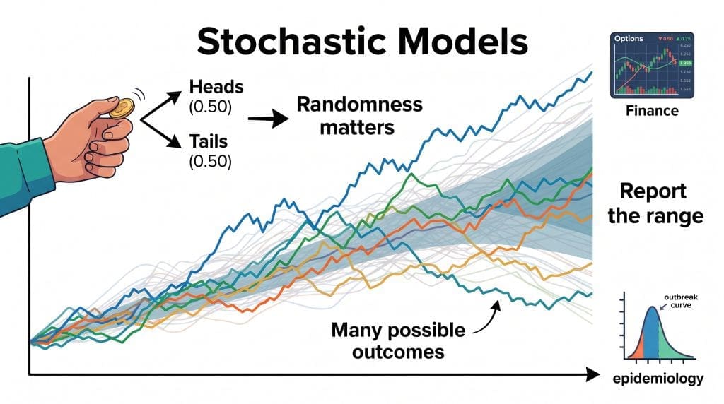
Stochastic models treat randomness as an integral part of the scenario; a random variable is used in place of a fixed value. Each possible value has a certain probability. Effectively, the model includes a noise term, where d W stands for Brownian motion. Consequence of this is that each instance differs from the previous one. For example, Monte Carlo methods involve repeating the model. A coin toss is the most straightforward way of imagining this. Indeed, each side has a known probability. Such techniques are employed in finance for pricing options and in epidemiology for modelling the spread of an outbreak. The advantage is that risk is portrayed honestly, not with false precision. On the other hand, the drawback is that it requires more effort. Because of this, analysts give a range. This range then informs risk decisions.

Generally speaking, combining both types of approach is the most effective strategy. Real-world systems combine certainty with randomness. Of course, clear reporting ensures that the ranges remain honest.
Real-World Mixes of Both
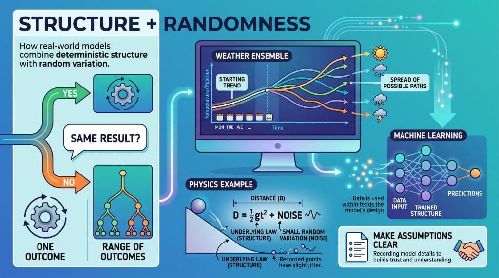
It is rare for a system to be entirely one or the other. Engineers often add noise to deterministic models, so the outcome retains both the general shape and the variation. Weather ensembles operate in this manner. Moreover, many physics equations begin with a simple form and then incorporate measurement errors via random terms. The final model thus belongs to both categories. In fact, machine learning takes this balance even further by relying on observed data; however, the training process still presumes a certain structure. Of course, the decision depends on the particular question. To be precise, one should consider whether one run produces exactly the same result. If the answer is yes, then the model should be kept deterministic. If not, probability should be introduced and a range of possible outcomes reported. Recording this choice is helpful to other researchers because it makes the assumptions clear.
In general, making assumptions explicit builds trust among readers. Ambiguous models, on the other hand, lead to subtle errors. In the end, transparency is more important than the label.
Dynamic, Static, Linear, and Non-linear Model Classes
Static and Dynamic Types of Mathematical Models
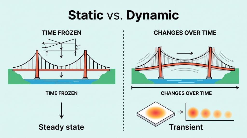
Static models ignore time and describe a system in a fixed state. For example, they can calculate the stress in a bridge under steady loads. Dynamic models, by contrast, show how a system changes over time. The heat equation is a common example because it describes how heat spreads through a region. Here, temperature depends on both position and time. Eventually, the system may reach a steady state, where conditions no longer change with time. Before that, it goes through a transient phase. Dynamic models capture these changes, while static models focus on a single state. Choosing the wrong model can hide important behaviour. For example, a static analysis may miss how a bridge bends under changing loads. Fluid flow problems follow the same principle. Steady-state solutions often require less computing time, while transient solutions reveal how a system responds to change. In short, each approach answers a different question.
Linear and Nonlinear Model Behavior
Linear models obey the superposition principle, which means that if the input is doubled the output is also doubled. They are usually easy to predict and solve. Simple regression and basic circuit models are typical examples. Nonlinear models, on the other hand, do not adhere to this principle. Feedback and thresholds can result in more complicated behavior. A case in point is the logistic map, which shows how a value changes through repeated steps. Minor changes in its parameter can cause greatly different outcomes, a characteristic associated with chaos theory. Climate models also exhibit nonlinear behaviour. Because superposition does not apply, solving such models may require greater computing power.
Physicists often make use of simpler approximations in order to obtain quick results and to detect general trends. Nevertheless, nonlinear methods are required when these approximations fail to capture important details. To sum up, the decision between using a linear and a nonlinear model depends on the system under investigation and the kind of behaviour that is to be understood.

Discrete and Continuous Types of Mathematical Models
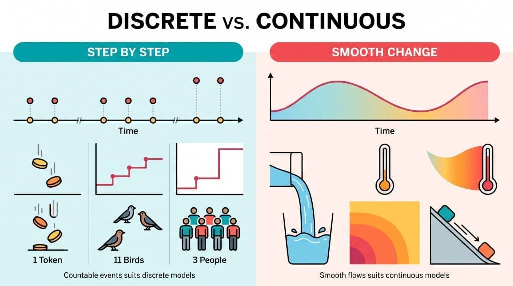
Discrete models involve separate and countable steps; time, for example, advances in jumps. Difference equations are good at describing such models. One example is that x next equals x squared plus c. On the other hand, continuous models rely on smooth change, and calculus is used to deal with that kind of smooth change. Discrete and continuous mathematical models usually go together, while agent-based models introduce a third type. In this case, each agent obeys simple local rules; traffic and epidemics are examples of this. A study has been verified which shows a link between discrete and continuous cell models, and age-structured vaccine planning has used the same mathematics.
In contrast, estimates allow one model to be substituted for the other. Therefore, the appropriate choice depends on the data; for instance, counted events are suitable for difference equations and, similarly, smooth flows are appropriate for differential equations. Overall, combining both types of model allows multiscale systems to be captured. To sum up, current software supports all these approaches. Of course, you should choose the one that corresponds to the readings you are working with, since this ensures that the results remain meaningful.
Master Comparison Table: All Model Types at a Glance
The table below gathers each class in one place. Read it as a decision aid, not a rulebook. For example, each row lists the domain and math. In fact, strengths and limits sit together. For instance, each entry ends with an example and use case. Comparing types of mathematical models gets faster this way. In practice, start with the matching column. At first, ask whether time matters for your system. Then check whether randomness plays a role. Finally, confirm the scale of your data. As a result, three answers narrow the field. A flowchart follows the table for visual learners. In short, use both tools together. Skipping this step invites silent errors. The wrong class can still produce charts. As a result, those charts answer the wrong question. Overall, that risk makes the effort worthwhile.
Table: 1 Master Comparison Table
| Type | Definition | Domain | Mathematics Used | Strengths | Limitations | Example | When to Use |
| Theoretical | Rule-based description from established principles | Physics, engineering | Differential equations, conservation laws | Clear, travels well | Needs correct assumptions | Newton’s second law | When the mechanism is known |
| Empirical | Pattern fitted to measured data | Economics, analytics | Regression, statistical fitting | Flexible, easy to update | Needs clean samples | Marketing response curves | When data are abundant |
| Deterministic | Same input always yields the same output | Mechanics, circuits | ODEs, PDEs, linear algebra | Repeatable, quick to solve | Ignores real-world randomness | Cooling coffee model | When variation is negligible |
| Stochastic | Outcomes vary through random variables | Finance, epidemiology | SDEs, Markov chains, Monte Carlo | Quantifies uncertainty | Heavier work | Option pricing models | When risk matters |
| Static | Time-free snapshot at equilibrium | Structural design | Algebraic equations | Simple and fast | Misses transient behaviour | Bridge stress analysis | When the system has settled |
| Dynamic | Tracks change through time | Climate, biology | Time-dependent ODEs and PDEs | Captures motion and feedback | Needs more data and compute | Heat equation | When change is the question |
| Structural | Shape set by linearity, discreteness, and scale | All fields | Superposition, difference equations | Matches problem structure | Wrong choice breaks solvers | Logistic map | When linearity or scale decides |
How Context Guides Model Class Choice and Regulatory Compliance
It is impossible to select a model class on the basis of numbers alone; in reality, it is the context that determines which assumptions are valid. Nowadays, watchdogs are requesting that modelling choices be recorded. The FDA has issued clear guidance regarding model credibility. Essentially, its approach links the evidence to the decision. For example, the national laboratories follow similar standards. As a result, the standard is raised. Consequently, recording the assumptions has become an integral part of the work. External reviewers are required to reproduce your results. Compared with this, having clear records makes it possible to carry out a review. To sum up, sorting also serves the purpose of communication since it allows people outside the team to check your reasoning.
Briefly put, good modelling is a collaborative activity. Teams that omit this step waste valuable review time. For instance, those groups that do record their assumptions are able to move more quickly. In the long run, this practice brings benefits throughout a person’s career. Of course, you should begin making the record before you write down the equations. During audits, reviewers check this line of thinking. A clear rationale helps to secure approval.

Two Simple Checks to Catch Modeling Errors Early
Most sorting errors can be caught using two checks. The first is to make sure the output agrees with the question; for instance, a model might appear accurate yet still be wrong. The second is to examine the assumptions in light of actual cases. Initially, you should apply the model to a known example; if it fails in that case, the model is incorrect. As a result, small-scale tests help to save substantial amounts of money since prototypes take only hours whereas full builds take months. In fact, this large difference shows that early testing is important.
Initially, you should keep a record of each failed attempt; by comparing the failures, the number of viable options is reduced. Over time, your judgement gets better. Experienced modelers are able to identify familiar patterns very quickly and can detect a misclassified case within minutes. Of course, you can develop this ability through practice. Reviewers place value on the documented record of the process. In short, this turns guesswork into a systematic approach and, through better habits, leads to better decisions. Overall, that is the real lesson.
Frequently Asked Questions About Model Types
Linear equations are the simplest thing to start with; they cause inputs to increase in a straight line and beginners are able to solve them by hand.
Simple models are solved using a pen and paper, while complex ones require numerical solvers; chaotic systems generally need machines.
Biology combines deterministic elements with stochastic ones; for example, population growth usually appears to be deterministic, while cellular noise must be treated in a stochastic way.
The results will vary depending on the assumptions made. Indeed, you should first look at the time frame and the element of randomness. Small decisions can cause a big change in the outcome.
Ask whether your system changes over time. If it settles, a static model suffices. Of course, moving systems need dynamic tracking.
How This Guide Was Compiled
We built this guide using reliable, reviewed sources. Each equation comes from standard textbooks, and we checked every reference against its publisher’s page. Only open-access papers made the final list. Government documents provided the relevant rules. We excluded vendor materials and blogs from the initial research. For example, definitions follow established engineering principles, while the categories reflect those used in modelling courses. We also compared our approach with two independent reviews. Where sources disagreed, we presented both perspectives. No claim relies on a single study. Readers can check the references themselves. We flagged one broken link and replaced it with a verified source. Transparency about sources helps build trust and supports current quality standards. Readers can send corrections through the nycstem.in’s contact page.
We organized the model classes around the questions they answer. Other sources group models by discipline or mathematical method. However, we chose a question-based structure because it reflects how practitioners select models. Each section explains its assumptions at the start. Standard references provide the examples, and consistent notation makes the guide easier to follow. Since different fields sometimes use different terms for the same idea, we added cross-links to connect related concepts. We also reduced unnecessary jargon without sacrificing accuracy. This approach helps beginners understand the material while allowing experts to find information quickly. Feedback from two readers helped us improve the wording. Their questions revealed unclear passages, and each revision made the definitions more precise. The final structure reflects this process of review and improvement.
Verified Resources
- U.S. Food and Drug Administration — modelling and simulation guidance.
- National Institute of Standards and Technology — applied and computational mathematics reports.
- Archives of Computational Methods in Engineering — peer-reviewed review articles.
- ScienceDirect — Computer Methods and Programs in Biomedicine
- Royal Society Open Science — open-access methodological studies.
- Axioms and Encyclopedia (MDPI) — open-access modelling research.
References:
Afzal, A., Saleel, C. A., Bhattacharyya, S., Satish, N., Samuel, O. D., & Badruddin, I. A. (2022). Merits and limitations of mathematical modeling and computational simulations in mitigation of COVID-19 pandemic: A comprehensive review. *Archives of Computational Methods in Engineering, 29*(2), 1311–1337. https://doi.org/10.1007/s11831-021-09634-2
Boisvert, R. F. (Ed.). (2023). *Applied and computational mathematics division: Summary of activities for fiscal year 2022* (NIST IR 8466). National Institute of Standards and Technology. https://doi.org/10.6028/NIST.IR.8466
Cheng, Z., & Wang, J. (2022). Modeling epidemic flow with fluid dynamics. *Mathematical Biosciences and Engineering, 19*(8), 8334–8360. https://doi.org/10.3934/mbe.2022388
González-Parra, G., Cogollo, M. R., & Arenas, A. J. (2022). Mathematical modeling to study optimal allocation of vaccines against COVID-19 using an age-structured population. *Axioms, 11*(3), 109. https://doi.org/10.3390/axioms11030109
Martinson, W. D., Volkening, A., Schmidtchen, M., Venkataraman, C., & Carrillo, J. A. (2024). Linking discrete and continuous models of cell birth and migration. *Royal Society Open Science, 11*(7), 232002. https://doi.org/10.1098/rsos.232002
Padmanabhan, R., Abed, H. S., Meskin, N., Khattab, T., Shraim, M., & Al-Hitmi, M. A. (2021). A review of mathematical model-based scenario analysis and interventions for COVID-19. *Computer Methods and Programs in Biomedicine, 209*, 106301. https://doi.org/10.1016/j.cmpb.2021.106301
Taite, G., & DiNapoli, J. (2025). Perspectives on mathematical modeling education: Conceptions and research. *Encyclopedia, 5*(3), 138. https://doi.org/10.3390/encyclopedia5030138
U.S. Food and Drug Administration. (2023). *Assessing the credibility of computational modeling and simulation in medical device submissions*. https://www.fda.gov/regulatory-information/search-fda-guidance-documents/assessing-credibility-computational-modeling-and-simulation-medical-device-submissions
Wang, J. (2020). Mathematical models for COVID-19: Applications, limitations, and potentials. *Journal of Public Health and Emergency, 4*, 9. https://doi.org/10.21037/jphe-2020-05